Exercises

This document contains instructions, some answers, comments, tips and tricks, and further explanations for the exercises.

In the first 6 exercises the answers start with identifying the population and parameter being studied.
In the answers I also mention the Test Statistic that can be used to test the hypothesis, although this is not requested. This is always a statistic of a sample used.

Exercise 9.1

Population: 1000 students with age 30+ at teachers’ college
Parameter: $\mu$: mean score for SSHA test

H₀: $\mu$ = 115
H_A: $\mu$ > 115

Test Statistic: $\bar{x}$, sample mean SSHA score in an SRS of 45 students at the teacher’s college aged 30+.

Note. I assume that ‘a better attitude’ leads to a higher SSHA score.

Exercise 9.2

Population: all Jordanian children
Parameter: $\mu$: mean amount of hemoglobin per deciliter of blood in g/dl

H₀: $\mu$ = 12
H_A: $\mu$ < 12

Test Statistic: $\bar{x}$, sample mean amount of hemoglobin in an SRS of 50 Jordanian children

Exercise 9.3

Population: all students at Simon’s college Parameter: p, proportion (or percentage) of left-handed persons

H₀: p = 0.12
H_A: p <> 0.12

Test Statistic: $\hat{p}$, proportion of left-handed people in an SRS of 100 students at Simon’s college

Exercise 9.4

Population: all teens at Yvonne’s highschool
Parameter: p, proportion that seldom or never argue with friends

H₀: p = 0.72
H_A: p <> 0.72

Test Statistic: $\hat{p}$, proportion students that seldom or never argue with friends in an SRS of 150 students at Yvonne’s highschool

Exercise 9.5

Population: thermostats manufactured by the manufacturer of Mrs. Starnes thermostat
Parameter: $\sigma$ standard deviation of the temperature if the thermostat is set at 50^oF.

H₀: $\sigma$ = 3
H_A: $\sigma$ > 3

Test Statistic: s, standard deviation in a randomly chosen couple of days on which the temperature was set on 50^oF.

As an alternative, use the Variance $\sigma$².

H₀: $\sigma$² = 9
H_A: $\sigma$² > 9

Exercise 9.6

Population: All ski jumpers that join the specific competition
Parameter: $\sigma$, the standard deviation of the distances in the jumps

H₀: $\sigma$ = 10
H_A: $\sigma$ > 10

Test Statistic: s, standard deviation in an SRS of jumps at the specific ski spring track

As an alternative, use the Variance $\sigma$².

Exercise 9.7

The form of the H₀ hypothesis always is H₀: parameter = ….
So in this case
p: proportion of all students atthe highschool that approve the parking situation
H₀: p = 0.37
H_a: p > 0.37 (greater than, because the test is performed to find support for an improved student satisfaction)

Exercise 9.8

$\hat{p}$ is a sample characteristic (a random variable)
Hypotheses are statements about a population parameter, not about a sample charateristic. For the correct hypotheses, see answer to 9.7

Exercise 9.9

$\bar{x}$ is a sample characteristic (a random variable)
Hypotheses are statements about a population parameter, not about a sample charateristic.

Correct hypotheses in this case:
$\mu$: average birth weight of all babies (in the US?) whose mothers didn’t see a doctor before delivery
H₀: $\mu$ = 1000 grams
H_a: $\mu$ <> 1000 grams

Note 1. Because nothing is said about the direction of the study, I use ‘is not equal to’ in the H_a.
Note 2. A little bit strange hypotheses, 1000 grams is a very low birth rate.

Exercise 9.10

The form of the H₀ hypothesis always is H₀: parameter = ….
So in this case:

$\mu$: average birth weight of all babies (in the US?) whose mothers didn’t see a doctor before delivery
H₀: $\mu$ = 1000 grams
The alternative has to use the value used in the H₀-hypotheses, so:
H_a: $\mu$ <> 1000 grams (or, depending on what is exactly been studied, H_a: $\mu$ < 1000 grams or H_a: $\mu$ > 1000 grams)

Exercise 9.11

Setting and hypotheses see 9.1. If H₀ is true, the average score for 30+ students at the college equals 115, so it doesn’t differ from the other students
Assuming that the average score for all 30+ students at the college is 115, the probability of an average score of 125.7 in an SRS from these 30+-students with n = 45 equals 0.0101.
Or, with $\mu$ the average score all 30+college students at the college and $\bar{x}$ the average score in an SRS of 45 30+-students at the college: P($\bar{x}$ <= 125.7 | $\mu$ = 115) = 0.0101

Exercise 9.12

If the H₀ hypothesis is true, than the average hemoglobin level for Jordanian children is 12 (g/dl); so on average Jordanian children are not anemic.
P-value = 0.016, this means that if the average hemoglobin level for Jordanian children indeed equals 12 (g/dl), the probability that in a SRS of 50 Jordanian children the mean hemoglobin level equals 11.3 (g/dl) or less is 0.0016.

Exercise 9.13

P-value = 0.2184
This means that if H₀ is true, the probability that a sample result will be found as Simon did or more extreme, is 0.2184. So the sample result is not unlikely.
If the significance level used, $\alpha$ = 0.10, H₀ will not be rejected.
If the significance level used, $\alpha$ = 0.05, H₀ will not be rejected.

In both cases the test doesn’t provide convincing evidence that the proportion of ‘lefties’ at SImon’s college differs from that of all adults in the US.

Exercise 9.14

Population: all teens at Yvonne’s highschool
Parameter: p, proportion that seldom or never argue with friends

H₀: p = 0.72
H_A: p <> 0.72

Test Statistic: $\hat{p}$, proportion students that seldom or never argue with friends in an SRS of 150 students at Yvonne’s highschool

Test result: 96 students out of 150 seldom or never argue with friends, $\hat{p}$ = $ = 0.64

P-value = 0.0291 (given)[^1]
If H₀ is true, the probability that the sample proportion is as extreme or more extreme than the observed one - that is in this case less than 0.64 or more than 0.80 - is 0.0291
If $\alpha$ = 0.05

Exercise 9.15

P-value = 0.0101 (given see exercise 9.11) if $\alpha$ = 0.05, H₀ is rejected, because P-value < $\alpha$
if $\alpha$ = 0.01, H₀ is not rejected, because P-value > $\alpha$

Exercise 9.16

P-value = 0.0016 (given see exercise 9.11) if $\alpha$ = 0.05, H₀ is rejected, because P-value < $\alpha$
if $\alpha$ = 0.01, H₀ is rejected, because P-value < $\alpha$

Exercise 9.17

H₀ is either true or false, that doesn’t depend on a sample result. The P-value is not the chance that the H₀ hypothesis true, but it is a conditional probability, P(a sample result as found or even more extreme in the direction of H_A | H₀ is true).

Exercise 9.18

The student forgets to mention that it is a conditional probability and that it is the probability $\hat{p}$ = 0.64 or more extreme in the diretion of the H_A hyoothesis.

Exercise 9.19

It is incorrect to compare the P-value with the proportion that is tested.
Besides that, data never prove that H_A is true, data can support the H_A hypothesis.

Exercise 9.20

Not rejecting H₀ is not the same as accepting H₀.
The conlucion should be, ‘because P-value is greater dan $\alpha$ = 0.05, we do not reject the H₀ hypothesis’.

Exercise 9.73

Part (a)

S(TATE)
$\mu$: the average speed of all drivers in the construction zone
H₀: $\mu$ = 25 mph H_A: $\mu$ > 25
$\alpha$ is not given; I will use $\alpha$ = 0.05

P(LAN)
Use a one-sample t-test for the mean, based on an SRS of 10 drivers to test the hypothesis.
Condtions:

Random sample? Yes.
10% condition? Yes, 10 drivers can be assumed less than 10% of all drivers in the zone.
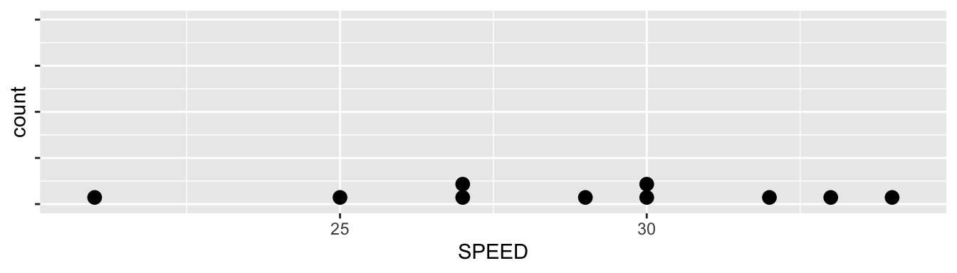
CLT? (that is the same as Normal/10% condition) Yes, see graph below. No extreme outliers and no skewness in the sample distribution, CLT can be used, i.e. it can be assumed that the sampling distribution of the sample mean is approximately normal.

D(O)
Perform the t-test, using TI84.

Output t-test in R

## 
##  One Sample t-test
## 
## data:  data$SPEED
## t = 3.0511, df = 9, p-value = 0.006884
## alternative hypothesis: true mean is greater than 25
## 95 percent confidence interval:
##  26.51697      Inf
## sample estimates:
## mean of x 
##      28.8

C(ONCLUDE)
From the output we see: p-value = 0.007
Because p-value < $\alpha$, H₀ is rejected in favor of H_A.
The data support the hypothesis that the average speed of all drivers at the construction zone exceeds 25 mph.

REMARK
It can be questioned whether in a practical sense this is the most interesting.
Maybe it is more interesting to state a hypothesis about the proportion of drivers who drive faster than 25 mph. To perform a test for a proportion, a sample with n=10 does not suffice, because with n = 10, one ‘success’ more or less makes a difference of 10%.

Part (b)

According to the theory:

a type I error means rejecting H₀ while it is actually true
a type II error means not rejectiong H₀ while H_A is actually true

This means that:

if H₀ is rejected, a type I error can be made
if H₀ is not rejected, a type II error can be made

In this case, H₀ is rejected, so a type I error can be made.
In the context this means, that based on the sample it is concluded that the average speed at the construction zone is more than 25 mph when in reality this is not true.