Handout week 48
AP Stats course Teacher: Hans van der Zwan Handout week 48
Literature Starnes D. S., et al. (2015). The Practice of Statistics (5th ed.). New York: W. H. Freeman and Company/BFW.
Handout per lesson
Lesson 1 Sun 2022-11-27
Learning Objectives
SKILL_ID | SKILL | TOPIC_ID | TOPIC | LO_ID | LEARNING_OBJECTIVE |
No STATS class today
Lesson 2 Mon 2022-11-28
Learning Objectives
SKILL_ID | SKILL | TOPIC_ID | TOPIC | LO_ID | LEARNING_OBJECTIVE |
3B | Determine parameters for probability distributions. | 4.8 | Mean and Standard Deviation of Random Variables | VAR-5C | Calculate parameters for a discrete random variable. [Skill 3.B] |
4B | Interpret statistical calculations and findings to assign meaning or assess a claim. | 4.8 | Mean and Standard Deviation of Random Variables | VAR-5D | Interpret parameters for a discrete random variable. [Skill 4.B] |
Preparation for lesson
See homework previous lesson
Theory
Topics: Random Variables; Expected Value and Standard Deviation Book: pp. 350-355
Class Activities
Lab
- Exercise 6.5, 6.7, 6.13
Discuss
- Standard Deviation of Random Variables; book pp. 352-353 and see example below
- Exercise 17
Expected Value of a Discrete Random Variable The probability distribution of a discrete random variable can be interpreted as ‘expected relative frequencies’ after repeating an experiment many, many times. This does not mean that it is expected to find exactly these probabilities as relative frequencies. It does mean that after repeating the experiment lots of times, the relative frequencies will be close to the probabilities. And according to the law of large number, the more often the experiment is repeated, the closer the experimental relative frequencies are to the probabilities. These expected relative frequencies have an expected mean value associated with them. This expected mean can be calculated as a weighted mean of the possible outcomes with the probabilities as weights. This expected mean value is called ‘the expected value’ of the random variable.
See example on pp. 350-351.
Example What is the expected value of X: the number that comes up when rolling a dice. First construct the probability distribution of X.
| x | 1 | 2 | 3 | 4 | 5 | 6 |
|---|---|---|---|---|---|---|
| P(X=x) | 1/6 | 1/6 | 1/6 | 1/6 | 1/6 | 1/6 |
Then calculate the Expected Value of X. E(X) = \(\mu_{X}\) = 1.1/6 + 2.1/6 + 3.1/6 + 4.1/6 + 5.1/6 + 6.1/6 = 3 1/2 Note: expected value is not what is expected if a dice is rolled, rolling 3 1/2 is even impossible. Expected value means that if a dice is rolled over en over again, the average value will approach 3 1/2. The more often the dice is rolled, the closer the average is to 3 1/2 (law of large numbers).
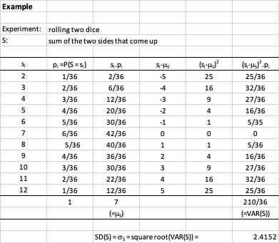
Variance and Standard Deviation of a Discrete Random Variable Probability Distributions can be visualized by graphs. Especially histograms are used a lot to visualize them. Based on a histogram, the distribution can be characterized using the SOCS method. The most common way to measure the centre of a probability distribution is by calculating the Expected Value. This is in fact the Mean value of the distribution. To measure the spread, the Standard Deviation (= square root of the Variance), is most commonly used. As with the Expected Value, to calculate the Variance, as in Chapter 1, calculate the average squared distance from the mean. This is the weighted average of the squared distances; the probabilities are the weights to be used. The Standard Deviation is the square root of the Variance. Formulas: \(VAR_X~=~\sum((x_i~-\mu_X)^2~\times~p_i)\) \(SD_X~=~\sqrt{VAR_X}=~\sqrt{\sum((x_i~-\mu_X)^2~\times~p_i)}\)
Example Experiment: rolling two dice S: sum of the two sides coming up The scheme below shows how the Expected Value and the Standard Deviation of S can be calculated. The TI84 can be used to do this as well, see book p. 354.
Homework
Study section 6.1. Exercises 6.27 to 6.30
Homework Assigment to hand in
-
Lesson 3 Tue 2022-11-29
Learning Objectives
SKILL_ID | SKILL | TOPIC_ID | TOPIC | LO_ID | LEARNING_OBJECTIVE |
2B | Construct numerical or graphical representations of distributions. | 4.7 | Introduction to Random Variables and Probability Distributions | VAR-5A | Represent the probability distribution for a discrete random variable. [Skill 2.B] |
3B | Determine parameters for probability distributions. | 4.8 | Mean and Standard Deviation of Random Variables | VAR-5C | Calculate parameters for a discrete random variable. [Skill 3.B] |
4B | Interpret statistical calculations and findings to assign meaning or assess a claim. | 4.7 | Introduction to Random Variables and Probability Distributions | VAR-5B | Interpret a probability distribution. [Skill 4.B] |
4B | Interpret statistical calculations and findings to assign meaning or assess a claim. | 4.8 | Mean and Standard Deviation of Random Variables | VAR-5D | Interpret parameters for a discrete random variable. [Skill 4.B] |
Preparation for lesson
See homework previous lesson
Theory
Topics: Wrap up Chapter 6 so far; Continuous Random Variables Book: Section 6.1
Class Activities
- Calculating Expected Value and Standard Deviation with the TI84
- Continuous Probability Distributions
- Uniform Distributions
- Normal Distributions
- recap; Chapter 2, pp. 108-128
- Frappy Question on p. 134
Lab
Exercise 2.42, 2.43, 2.53
Homework
Repeat theory about Normal Distributions, pp. 108-128 Exercises 2.42, 2.43, 2.53
Homework Assigment to hand in
-
Lesson 4 Wed 2022-11-30
Learning Objectives
SKILL_ID | SKILL | TOPIC_ID | TOPIC | LO_ID | LEARNING_OBJECTIVE |
3B | Determine parameters for probability distributions. | 4.9 | Combining Random Variables | ||
3C | Describe probability distributions. | 4.9 | Combining Random Variables |
Theory
Topic: Transforming Random Variables Book: pp. 363-368
Preparation for lesson
See homework previous lesson
Class Activities
Discuss
- Influence of linear transformations on the Expected Value and Standard Deviation of a Random Variable
Rule 1 If X is a discrete random variable and Y = X + c (c a constant), then: \(\mu_Y=\mu_X+c\) and \(\sigma_Y=\sigma_X\) and \(VAR_Y~=~VAR_X\)
Rule 2 If X is a discrete random variable and Y = cX (c a constant), then: \(\mu_Y= c \times \mu_X\) and \(\sigma_Y= c \times \sigma_X\) and \(VAR_Y~=~c^2~\times~VAR_X\)
Rule 3: combining rule 1 and rule 2 If X is a discrete random variable and Y = a + bX (a and b constants), in other words Y is constructed by applying a linear transformation to X, then: \(\mu_Y= a + b \times\mu_X\) and \(\sigma_Y= b \times\sigma_X\) and \(VAR_Y~=~b^2~\times~VAR_X\)
Example The relationship between temperature in \(^0F\) and \(^0C\) is: \(Temperatuur~in~^0F~=~32~+~\frac{9}{5}\times~Temperature~in~^0C\)
Define the random variable T: the maximum temperature in Amman on a randomly chosen day in October in degrees Celsius. Based on historical data, \(\mu_T = 28.6^0C\) and \(\sigma_T = 4.0^0C\). The random variable F is defined as the maximum temperature in Amman on a randomly chosen day in October in degrees Fahrenheit. The question is, what are \(\mu_F\) and \(\sigma_F\)? Applying the rule3: \(\mu_F~=~32~+\frac{9}{5}~\times~\mu_X~=~32~+\frac{9}{5}~\times~28.6~=~83.5~^0F\) \(\sigma_F~=~\frac{9}{5}~\times~\sigma_X~=~\frac{9}{5}~\times~4.0~=~7.2^0F\)
Figure 48.1 Maximum Daily Temperatures in October in Amman, 1979 to 2013
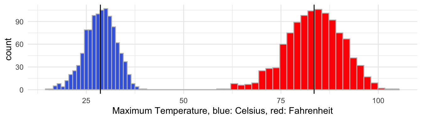
Note. The black lines indicate the mean in \(^0\)C resp. \(^0\)F. As can be seen the average value in \(^0\)F is 32 more than the average in \(^0\)C. The spread of the vales in \(^0\)F is a factor \(\frac{9}{5}\) higher than the spread of the values in \(^0\)C.
Homework
Prepare for test about Chapter 5
Homework Assigment to hand in
-
Lesson 5 Thu 2022-12-01
Learning Objectives
SKILL_ID | SKILL | TOPIC_ID | TOPIC | LO_ID | LEARNING_OBJECTIVE |
1A | Identify the question to be answered or problem to be solved (not assessed). | 4.1 | Introducing Statistics: Random and Non-Random Patterns? | VAR-1.F | Identify questions suggested by patterns in data. [Skill 1.A] |
3A | Determine relative frequencies, proportions, or probabilities using simulation or calculations. | 4.2 | Estimating Probabilities Using Simulation | UNC-2.A | Estimate probabilities using simulation. [Skill 3.A] |
3A | Determine relative frequencies, proportions, or probabilities using simulation or calculations. | 4.3 | Introduction to Probability | VAR-4.A | Calculate probabilities for events and their complements. [Skill 3.A] |
3A | Determine relative frequencies, proportions, or probabilities using simulation or calculations. | 4.5 | Conditional Probability | VAR-4.D | Calculate conditional probabilities. [Skill 3.A] |
3A | Determine relative frequencies, proportions, or probabilities using simulation or calculations. | 4.6 | Independent Events and Unions of Events | VAR-4.E | Calculate probabilities for independent events and for the union of two events. [Skill 3.A] |
4B | Interpret statistical calculations and findings to assign meaning or assess a claim. | 4.3 | Introduction to Probability | VAR-4.B | Interpret probabilities for events. [Skill 4.B] |
4B | Interpret statistical calculations and findings to assign meaning or assess a claim. | 4.4 | Mutually Exclusive Events | VAR-4.C | Explain why two events are (or are not) mutually exclusive. [Skill 4.B] |
Preparation for lesson
Chapter 5
Class Activities
Test Chapter 5